Microsoft Word - IsoCalcs30Sept04.doc

An Introduction to Isotopic Calculations

John M. Hayes (jhayes@whoi.edu)

Woods Hole Oceanographic Institution, Woods Hole, MA 02543, USA, 30 September 2004

Abstract. These notes provide an introduction to:

• Methods for the expression of isotopic abundances,

• Isotopic mass balances, and

• Isotope effects and their consequences in open and

closed systems.

Notation. Absolute abundances of isotopes are com-

monly reported in terms of atom percent. For example,

atom percent

C = [

C/(

C +

C)]100 (1)

A closely related term is the fractional abundance

fractional abundance of

C ≡

C/(

C +

C) (2)

These variables deserve attention because they provide

the only basis for perfectly accurate mass balances.

Isotope ratios are also measures of the absolute abun-

dance of isotopes; they are usually arranged so that the

more abundant isotope appears in the denominator

“carbon isotope ratio” =

C ≡

R (3)

For elements with only two stable nuclides (H, C, and N,

for example), the relationship between fractional abun-

dances and isotope ratios is straightforward

R =

F/(1 -

F) (4)

F =

R/(1 +

R) (5)

Equations 4 and 5 also introduce a style of notation.

In mathematical expressions dealing with isotopes, it is

convenient to follow the chemical convention and to use

left superscripts to designate the isotope of interest, thus

avoiding confusion with exponents and retaining the

option of defining subscripts. Here, for example, we

have written

F rather than F

or F

Parallel version of equations 4 and 5 pertain to multi-

isotopic elements. In the case of oxygen, for example,

1817

1 −−

(4a)

1817

1 ++

(5a)

Natural variations of isotopic abundances. The

isotopes of any element participate in the same chemical

reactions. Rates of reaction and transport, however,

depend on nuclidic mass, and isotopic substitutions

subtly affect the partitioning of energy within molecules.

These deviations from perfect chemical equivalence are

termed isotope effects. As a result of such effects, the

natural abundances of the stable isotopes of practically

all elements involved in low-temperature geochemical

(< 200°C) and biological processes are not precisely con-

stant. Taking carbon as an example, the range of interest

is roughly 0.00998 ≤

F ≤ 0.01121. Within that range,

differences as small as 0.00001 can provide information

about the source of the carbon and about processes in

which the carbon has participated.

The delta notation. Because the interesting isotopic

differences between natural samples usually occur at and

beyond the third significant figure of the isotope ratio, it

has become conventional to express isotopic abundances

using a differential notation. To provide a concrete

example, it is far easier to say – and to remember – that

the isotope ratios of samples A and B differ by one part

per thousand than to say that sample A has 0.3663 %

and sample B has 0.3659 %

N. The notation that pro-

vides this advantage is indicated in general form below

[this means of describing isotopic abundances was first

used by Urey (1948) in an address to the American

Association for the Advancement of Science, and first

formally defined by McKinney et al. (1950)]

STD

= 1

STD

Sample

−

(6)

Where

expresses the abundance of isotope A of ele-

ment X in a sample relative to the abundance of that

same isotope in an arbitrarily designated reference mater-

ial, or isotopic standard. For hydrogen and oxygen, that

reference material was initially Standard Mean Ocean

Water (

SMOW). For carbon, it was initially a particular

calcareous fossil, the PeeDee Belemnite (

PDB; the same

standard served for oxygen isotopes in carbonate miner-

als). For nitrogen it is air (

AIR). Supplies of PDB and of

the water that defined

SMOW have been exhausted. Prac-

tical scales of isotopic abundance are now defined in

terms of surrogate standards distributed by the Interna-

tional Atomic Energy Authority’s laboratories in Vienna.

Accordingly, modern reports often present values of

VSMOW

and

VPDB

. These are equal to values of

SMOW

and

PDB

The original definition of

(McKinney et al., 1950)

multiplied the right-hand side of equation 6 by 1000.

Isotopic variations were thus expressed in parts per thou-

sand and assigned the symbol ‰ (permil, from the Latin

per mille by analogy with per centum, percent). Equa-

tions based on that definition are often littered with

factors of 1000 and 0.001. To avoid this, it is more con-

venient to define δ as in equation 6. According to this

view (represented, for example, by Farquhar et al., 1989

and Mook, 2000), the ‰ symbol implies the factor of

1000 and we can equivalently write either

= -25‰ or

= -0.025.

To avoid clutter in mathematical expressions, sym-

bols for

should always be simplified. For example,

can represent

PDB

(

HCO ). If multiple elements and

isotopes are being discussed, variables like

and

are explicit and allow use of right subscripts for desig-

nating chemical species.

Mass-Balance Calculations. Examples include (i)

the calculation of isotopic abundances in pools derived

by the combination of isotopically differing materials,

(ii) isotope-dilution analyses, and (iii) the correction of

experimental results for the effects of blanks. A single,

master equation is relevant in all of these cases. Its

concept is rudimentary: Heavy isotopes in product =

Sum of heavy isotopes in precursors. In mathematical

terms:

= m

+ m

+ ... (7)

where the m terms represent molar quantities of the ele-

ment of interest and the F terms represent fractional iso-

topic abundances. The subscript Σ refers to total sample

derived by combination of subsamples 1, 2, ... etc. The

same equation can be written in approximate form by

replacing the Fs with δs. Then, for any combination of

isotopically distinct materials:

= Σm

/Σm

(8)

Equation 8, though not exact, will serve in almost all

calculations dealing with natural isotopic abundances.

The errors can be determined by comparing the results

obtained using equations 7 and 8. Taking a two-

component mixture as the simplest test case, errors are

found to be largest when

differs maximally from both

and

, i. e., when m

= m

. For this worst case, the

error is given by

Σ*

= (R

STD

)[(

)/2]

(9)

Where

is the result obtained from eq. 8;

Σ*

is the

exact result, obtained by converting

and

to frac-

tional abundances, applying eq. 7, and converting the

result to a

value; and R

STD

is the isotopic ratio in the

standard that establishes the zero point for the

scale

used in the calculation. The errors are always positive.

They are only weakly dependent on the absolute value of

and become smaller than the result of eq. 9 as

>> 0. If R

STD

is low, as for

H (

VSMOW

= 1.5 × 10

-4

the errors are less than 0.04‰ for any |

| ≤ 1000‰.

For carbon (

PDB

= 0.011), errors are less than 0.03‰

for any |

| ≤ 100‰.

The excellent accuracy of eq. 8 does not mean that all

simple calculations based on

will be similarly accurate.

As noted in a following section, particular care is

required in the calculation and expression of isotopic

fractionations. And, when isotopically labeled materials

are present, calculations based on

should be avoided in

favor of eq. 7.

Isotope dilution. In isotope-dilution analyses, an

isotopic spike is added to a sample and the mixture is

then analyzed. The original “sample” might be a

material from which a representative subsample could be

obtained but which could not be quantitatively isolated

(say, total body water). For the mixture (Σ) of the

sample (x) and the spike (k), we can write:

+ m

= m

+ m

(10)

Rearrangement yields an expression for m

(e. g., moles

of total body water) in terms of m

, the size of the spike,

and measurable isotopic abundances:

= m

- F

)/(F

- F

) (11)

Since we are dealing here with a mass balance,

can be

substituted for F unless heavily labeled spikes are

involved.

Blank corrections. When a sample has been con-

taminated during its preparation by contributions from an

analytical blank, the isotopic abundance actually deter-

mined during the mass spectrometric measurement is that

of the sample plus the blank. Using Σ to represent the

sample prepared for mass spectroscopic analysis and x

and b to represent the sample and blank, we can write

= m

+ m

(12)

Substituting m

= m

- m

and rearranging yields

- m

(

)/n

(13)

an equation of the form y = a + bx. If multiple analyses

are obtained, plotting

vs. 1/m

will yield the accurate

(i. e., blank-corrected) value of

as the intercept.

Calculations related to isotope effects

An isotope effect is a physical phenomenon. It

cannot be measured directly, but its consequences – a

partial separation of the isotopes, a fractionation – can

sometimes be observed. This relationship is indicated

schematically in Figure 1.

Fractionation. Two conditions must be met before

an isotope effect can result in fractionation. First, the

system in which the isotope effect is occurring must be

arranged so that an isotopic separation can occur. If a

reactant is transformed completely to yield some pro-

duct, an isotopic separation which might have been

visible at some intermediate point will not be observable

because the isotopic composition of the product must

eventually duplicate that of the reactant. Second, since

isotope effects are small enough that they don’t upset

blanket statements about chemical properties, the tech-

niques of measurement must be precise enough to detect

very small isotopic differences.

Observed fractionations are proportional to the mag-

nitudes of the associated isotope effects. Examples of

equilibrium and kinetic isotope effects are shown in

Figure 2. As indicated, the magnitude of an equilibrium

isotope effect can be represented by an equilibrium con-

stant. In this example, the reactants and products are

chemically identical (carbon dioxide and bicarbonate in

each case). However, due to the isotope effect, the equi-

librium constant is not exactly 1. There is, however, a

problem with the use of equilibrium constants to quantify

isotope effects. An equilibrium constant always pertains

to a specific chemical reaction, and, for any particular

isotopic exchange, the reaction can be formulated in

various ways, for example:

O + 1/3 CaC

' H

O + 1/3 CaC

(14)

vs.

O + CaC

' H

O + CaC

(15)

To avoid such ambiguities, EIEs are more commonly

described in terms of fractionation factors.

A fractionation factor is always a ratio of isotope

ratios. For the example in Figure 2, the fractionation

factor would be:

HCO

CO/HCO

⎟

⎠

⎞

⎜

⎝

⎛

⎟

⎠

⎞

⎜

⎝

⎛

−

(16)

A more compact and typical representation would be

b/g

= R

(17)

Here, subscripts have been used to designate the

chemical species (b for bicarbonate, g for gas-phase

) and the superscript 13 indicates that the exchange

C is being considered. The resulting equation is

more compact. It does not combine chemical and math-

ematical systems of notation and, as a result, is less

cluttered and more readable. For either reaction 14 or

15, the fractionation factor would be

c/w

= R

(18)

where c and w designate calcite and water, respectively.

For a kinetic isotope effect, the fractionation factor is

equal to the ratio of the isotope-specific rate constants. It

is sometimes denoted by

rather than

. In physical

organic chemistry and enzymology, however,

is gener-

ally reserved for the ratio of isotope-specific equilibrium

constants while

stands as the observed isotopic frac-

tionation factor.

There are no firm conventions about what goes in the

numerator and the denominator of a fractionation factor.

For equilibrium isotope effects it’s best to add subscripts

in order to indicate clearly which substance is in the

numerator and, for kinetic isotope effects, readers must

examine the equations to determine whether an author

has placed the heavy or the light isotope in the

numerator.

Reversibility and systems. Given a fractionation

factor, isotopic compositions of reactants and products

can usually be calculated once two questions have been

answered:

1. Is the reaction reversible?

2. Is the system open or closed?

Figure 2. Examples of equilibrium and kinetic

isotope effects.

Figure 1. Schematic representation of the relation-

ship between an isotope effect (a physical phenom-

enon) and the occurrence of isotopic fractionation (an

observable quantity).

An open system is one in which both matter and energy

are exchanged with the surroundings. In contrast, only

energy crosses the boundaries of a closed system.

Reversibility and openness vs. closure are key con-

cepts. Each is formally crisp, but authors often sew

confusion. If a system is described as “partially closed,”

readers should be on guard. If the description means that

only some elements can cross the boundaries of the

system, the concept might be helpful. If partial closure

instead refers to impeded transport of materials into and

out of the system, the concept is invalid and likely to

cause problems.

Openness covers a range of possibilities. Some open

systems are at steady state, with inputs and outputs

balanced so that the inventory of material remains

constant. In others, there are no inputs but products are

lost as soon as they are created. These cases can be

treated simply, others require specific models.

Reversible reaction, closed system. In such a

system, (1) the isotopic difference between products and

reactants will be controlled by the fractionation factor

and (2) mass balance will prevail.

To develop a quantitative treatment, we will consider

an equilibrium between substances A and B,

' B (19)

The isotopic relationship between these materials is

defined in terms of a fractionation factor:

A/B

(20)

where the Rs are isotope ratios and the

s are the

corresponding

values on any scale of abundances (the

same scale must be used for both the product and the

reactant). The requirement that the inventory of mater-

ials remain constant can be expressed inexactly, but with

good accuracy, in terms of a mass-balance equation:

= f

+ (1 – f

)

(21)

where

refers to the weighted-average isotopic com-

position of all of the material involved in the equilibrium

(for equation 14 or 15, it would refer to all of the oxygen

in the system) and f

refers to the fraction of that

material which is in the form of B. By difference, the

fraction of material in the form of A is 1 – f

Rearrangement of equation 20 yields:

A/B

+ (

A/B

– 1) (22)

The second term on the right-hand side of this equation

is commonly denoted by a special symbol:

- 1 ≡

(23)

Equation 22 then becomes:

A/B

(24)

(Like

is often expressed in parts per thousand. For

example, if

= 1.0077, then

= 0.0077 or 7.7‰.

Dimensional analysis reliably indicates the form required

in any calculation. In equations 24-29, all terms could be

dimensionless or could be expressed in permil units.

The dimensionless form is required in equation 20,

where

is added to a dimensionless constant, in equa-

tions 39 and 40, where use of permil units would unbal-

ance the equations, and in equations 41 and 42, where

and/or

appear as exponents or in the arguments of

transcendental functions.)

Substituting for δ

in equation 21, we obtain

= f

+ (1 – f

)(

A/B

) (25)

Solving for δ

, we obtain an expression which allows

calculation of δ

as a function of f

, given

A/B

and

BBA/B

A/BB

f)f(

)f(

+−

−

(26)

If equation 24 is rearranged to express

in terms of

A/B

, and

A/B

, and the result is substituted for

equation 21, we obtain a complementary expression for

BBA/B

A/BBA/B

)1( ff

+−

εδα

(27)

Equations 26 and 27 are generally applicable but

rarely employed because adoption of the approximation

A/B

≈ 1 yields far simpler results, namely:

+ f

A/B

(28)

and

- (1 – f

)

A/B

(29)

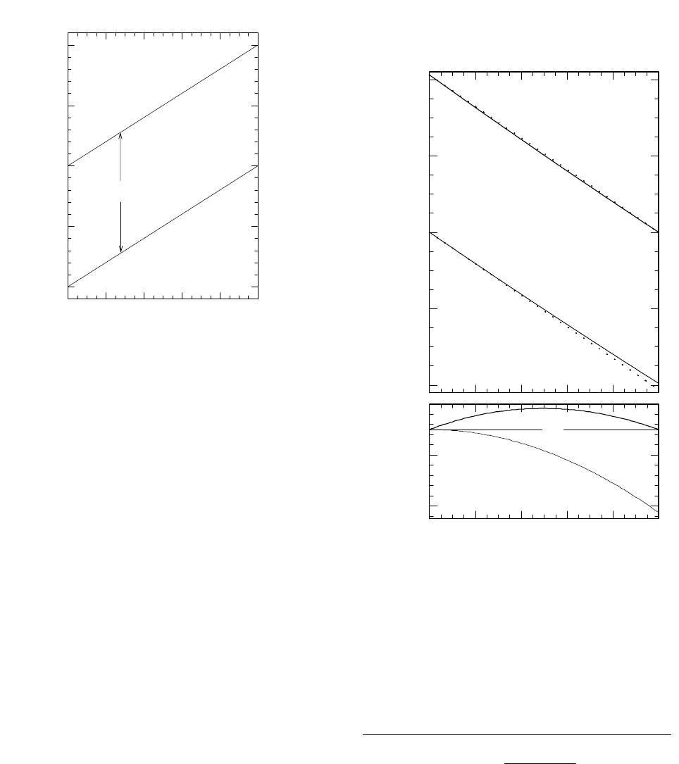
Graphs depicting these relationships can be constructed

very easily. An example is shown in Figure 3. For f

1 we must have

and for f

= 0 we must have

. As shown in Figure 3, the intercepts for the other

ends of the lines representing

and

will be

A/B

. If

A/B

< 1,

A/B

will be negative and A will be

isotopically depleted relative to B. The lines represent-

ing

and

will slope upward as f

→ 0. If

A/B

> 1

then A would be enriched relative to B and the lines

would slope downward.

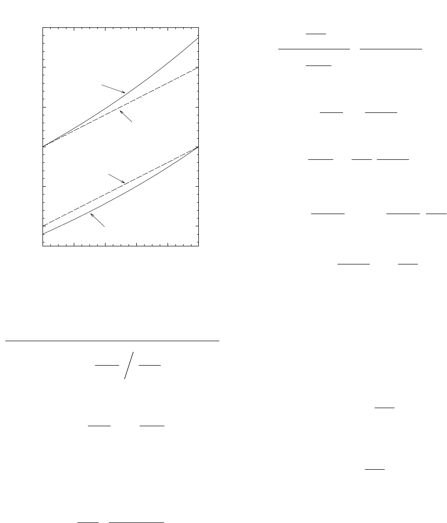
There are two circumstances in which the approxi-

mation leading to equations 28 and 29 (i. e.,

A/B

≈ 1)

must be examined. The first involves highly precise stu-

dies and the second almost any hydrogen-isotopic frac-

tionations. As an example of the first case, Figure 4

compares the results of equations 26 and 27 to those of

28 and 29 for a system with

A/B

= 1.0412. This is, in

fact, the fractionation factor for the exchange of oxygen

between water and gas-phase carbon dioxide at 25°C

(where A is CO

and B is H

O). The solid and dotted

lines in the larger graph represent the more accurate and

the approximate results, respectively. The lines in the

smaller graph in Figure 4 represent the errors, which

significantly exceed the precision of measurement

(which is typically better than 0.1‰).

For many hydrogen-isotopic fractionations,

differs

from 1.0 by more than 10%. In such cases, the approxi-

mation fails and a magnifying lens is not needed to see

the difference between the accurate and the approximate

results. An example is shown in Figure 5.

Irreversible reaction, closed system. The goal is to

determine the isotopic relationship between the reactants

and products over the course of the reaction, starting

with only reactants and ending with a 100% yield of

products. We’ll consider the general reaction R → P

(Reactants → Products). If the rate is sensitive to

isotopic substitution, we’ll have

P/R

≠ 1, where

P/R

≡ R

P,i

(30)

In this equation,

P/R

is the fractionation factor, R

P,i

the isotope ratio (e. g.,

C) of an increment of

product and R

is the isotope ratio of the reactant at the

same time. Following the approach of Mariotti et al.

(1981) and expressing R

P,i

in terms of differential quan-

tities, we can write

lRhR

lPhP

P/R

m/m

(31)

where the ms represent molar quantities and the sub-

scripts designate the

heavy and light isotopic species of

the

Product and Reactant. In absence of side reactions,

= -dm

and dm

= -dm

. Employing these

substitutions, the equation can be expressed entirely in

terms of quantities of reactant:

0.00.20.40.60.81.0

- ε

A/B

+ ε

A/B

, ‰

Figure 3. General form of a diagram depicting iso-

topic compositions of species related by a reversible

chemical reaction acting in a closed system.

0.00.20.40.60.81.0

+ ε

A/B

- ε

A/B

, ‰

Figure 4. Graphs showing results of both accurate

and approximate calculations of isotopic composi-

tions of reactants and products of a reversible reac-

tion in a closed system. The dotted lines in the upper

graph are drawn as indicated in Figure 3 and by equa-

tions 28 and 29. The solid lines are based on equa-

tions 26 and 27. The differences between these treat-

ments are shown in the smaller graph.

0.00.20.40.60.81.0

, ‰

-40

-20

A/B

= 1.0412

= 0

0.00.20.40.60.81.0

Error, ‰

-1.5

-0.5

0.5

⎟

⎠

⎞

⎜

⎝

⎛

⎟

⎠

⎞

⎜

⎝

⎛

P/R

(32)

Separating variables and integrating from initial condi-

tions to any arbitrary point in the reaction, we obtain

⎟

⎠

⎞

⎜

⎝

⎛

⎟

⎠

⎞

⎜

⎝

⎛

hR,0

lR,0

P/R

ln ln

(33)

where the subscript zeroes indicate quantities of

R and

R at time = 0.

It is convenient to define f as the fraction of reactant

which remains unutilized (i. e., 1 - f is the fractional

yield). Specifically:

lR,0hR,0

lRhR

R,0

(34)

Avoiding approximations introduced by Mariotti et al.

(1981), we rearrange this equation to yield exact substi-

tutions for the arguments of the logarithms in equation

33. For example:

⎟

⎠

⎞

⎜

⎝

⎛

⎟

⎠

⎞

⎜

⎝

⎛

)1(

R,0lR,0

RlR

lR,0

hR,0

lR,0

(35)

Which yields

R,0

lR,0

⋅=

(36)

Similar rearrangements yield

R,0

hR,0

⋅=

(37)

So that equation 33 becomes

⎟

⎠

⎞

⎜

⎝

⎛

⋅

⋅=

⎟

⎠

⎞

⎜

⎝

⎛

⋅

R,0

R,0R,0

P/R

(38)

Which can be rearranged to yield

⎟

⎠

⎞

⎜

⎝

⎛

⎟

⎠

⎞

⎜

⎝

⎛

⋅

R,0

P/R

(39)

an expression which duplicates exactly equation V.17 in

the rigorous treatment by Bigeleisen and Wolfsburg

(1958). Without approximation, this equation relates the

isotopic composition of the residual reactant (R

) to that

of the initial reactant (R

R,0

), to the isotope effect (

P/R

and to f, the extent of reaction.

If the abundance of the rare isotope is low, the

coefficient for f, (1 + R

R,0

)/(1 + R

), is almost exactly 1.

In that case, equation 39 becomes

R,0

P/R

ln ln

f =

(40)

Because quantities with equal logarithms must them-

selves be equal, we can write

R,0

P/R

f =

(41)

Equation 41 is often presented as “The Rayleigh Equa-

tion.” It was developed by Lord Rayleigh (John William

Strutt, 1842-1919) in his treatment of the distillation of

liquid air and was exploited by Sir William Ramsey

(1852-1916) in his isolation first of argon and then of

neon, krypton, and xenon. The ratios in these cases were

not isotopic. The concept of isotopes was introduced by

Frederick Soddy (1877-1956) in 1913, long after Strutt

and Ramsey had been awarded the Nobel Prizes in phys-

ics and chemistry, respectively, in 1904. Instead, the

ratios in Rayleigh’s conception pertained to the abun-

0.00.20.40.60.81.0

, ‰

-100

100

200

300

400

Accurate δ

Approximate δ

Accurate δ

A/B

= 0.800

= +100‰

Figure 5. Graph depicting isotopic compositions

of reactants and products of a reversible reaction in a

closed system with an α value typical of hydrogen

isotope effects.

dances of Ar, Ne, Kr, and Xe relative to N

and, as the

distillation proceeded, relative to each other.

Figure 6 indicates values of R

that are in accordance

with equation 41 (viz., the line marked R; on the

horizontal axis, “yield of P” = 1 – f). If the objective is

to use observed values of

and/or

in order to

evaluate

P/R

, a linear form is often desirable. One

which is linear and exact is provided by equation 39.

Values of

must be converted to isotope ratios and the

initial composition of the reactant must be known.

Regression of ln(R

R,0

) on ln[f(1 + R

R,0

)/(1 + R

)]

will then yield

P/R

as the slope.

By use of approximations, Mariotti et al. (1981)

developed less cumbersome forms. The first is derived

by rewriting equation 40 with the argument of the

logarithm in the delta notation. Rearrangement then

yields

()

(

)

fln1ln1ln

P/RR,0R

++=+ (42)

This is an expression of the form y = a + bx. Regression

of ln(

+ 1) on lnf yields a straight line with slope

P/R

A second form is very widely applied. Noting that

ln[(1 + u)/(1 + v)] ≅ u – v when u and v are small relative

to 1, Mariotti et al. (1981) simplified eq. 42 to obtain

R,0

P/R

·lnf (43)

This is also an expression of the form y = a + bx. More-

over, it is an equation in which all terms can be expres-

sed in permil units. Regression of

on lnf will yield

P/R

as the slope and

R,0

, which need not be known

independently, as the intercept.

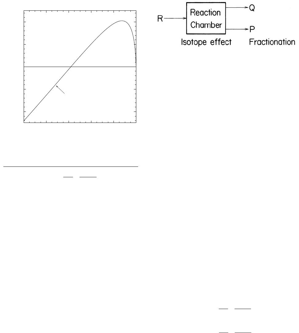
The approximations leading to equations 42 and 43

can lead to systematic errors. These are examined in

Figure 7, which is based on values of

and

that are

typical for

C. Equation 42 is based on the approxi-

mation that m

lR,0

does not differ significantly from

R,0

(cf. eq. 34). This is evidently much more

satisfactory than the approximation leading to equation

43, which produces systematic errors that are larger than

analytical uncertainties for values of f < 0.4. Equation 43

should never be used in hydrogen-isotopic calculations,

for which the approximation u ≈ v << 1 is completely

invalid.

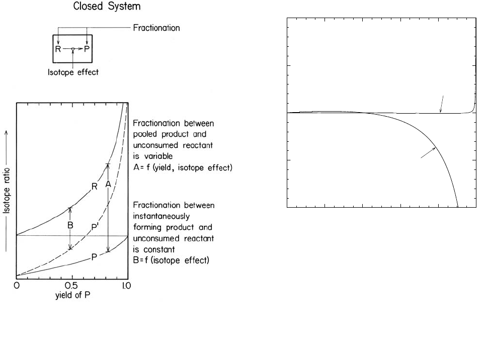
Equations 39-43 pertain to values of

, the isotopic

composition of the reactant available within the closed

system. Figure 6 also shows lines marked

P and P′ rep-

resenting respectively the isotopic compositions of the

pooled product and of the product forming at any point

in time. The relationship between R and P′ always

follows directly from the fractionation factor:

Figure 6. Schematic representation of isotopic

compositions of reactants and products for an irrever-

sible reaction in a closed system.

0.00.20.40.60.81.0

Error in

, ‰

-2

-1

Equation 43

Equation 42

P/R

= -30‰ (eq. 43) = -0.030 (eq. 42)

R,0

= -8‰ (eq. 43) = -0.008 (eq. 42)

STD

= 0.011180

Figure 7. Errors in values of

calculated using

equations 42 and 43.

P/R

′′

(44)

As noted in Figure 6, this leads to a constant isotopic

difference (designated

B in the Figure) between R and P′.

Initially, both the pooled product, P, and P′ are depleted

relative to R by the same amount. As the reaction pro-

ceeds, the isotopic composition of P steadily approaches

that of the initial reactant. The functional relationship

can be derived from a mass balance:

R,0

= m

+ m

(45)

substituting m

R,0

= f and m

R,0

= 1 - f, combina-

tion of equations 43 and 45 yields

R,0

– [f/(1 – f)]

P/R

·lnf (46)

an expression which shows that the regression of

[f/(1 – f)]·lnf will yield

P/R

as the slope.

Systematic errors associated with equation 46, sum-

marized graphically in Figure 8, are smaller than those in

equation 43 (note the differing vertical scales in Figs. 7

and 8).

In practical studies of isotope effects, the most vexing

problem is usually not whether to accept approximations

but instead how to combine observations from multiple

experiments. The problem has been explored systemati-

cally and very helpfully by Scott et al. (2004), who have,

in addition, concluded that calculations based on equa-

tion 42 are most likely to provide the smallest uncertain-

ties. Notably, they recommend regression of lnf on ln(

+ 1), thus necessitating transformation of the regression

constants in order to obtain a value for

P/R

. Although

both f and

are subject to error, use of a Model I linear

regression, and thus assuming that errors in

are small

in comparison to those in f, is recommended.

Reversible reaction, open system (product lost).

Atmospheric moisture provides the classical example of

systems of this kind. Water vapor condenses to form a

liquid or solid which precipitates from the system.

Vapor pressure isotope effects lead to fractionation of the

isotopes of both H and O. The process of condensation

is reversible, but the evolution of isotopic compositions

is described by the same equations introduced above to

describe fractionations caused by an irreversible reaction

in a closed system. The heavy isotopes accumulate in

the condensed phases. Consequently, the residual reac-

tant (the moisture vapor remaining in the atmosphere) is

described by increasingly negative values of

. The

curves describing the isotopic compositions have the

same shape as those in Figure 6, but bend downward

rather than upward.

Reversible or irreversible reaction, open system at

steady state.

A schematic view of a system of this kind

is shown in Figure 9. A reactant, R, flows steadily into a

stirred reaction chamber. Products P and Q flow from

the chamber. The amount of material in the reaction

chamber is constant and, therefore,

QPR

JJJ +

(47)

Where J is the flux of material, moles/unit time.

The relevant fractionation factors are

R/P

(48)

and

R/Q

(49)

It doesn’t matter whether these fractionations result from

reversible equilibria or from kinetically limited processes

that operate consistently because residence times within

the reactor are constant. As a result of these processes,

the isotopic difference between P and Q can also be

described by a fractionation factor

0.00.20.40.60.81.0

Error in

, ‰

-0.2

-0.1

0.0

0.1

0.2

Equation 46

P/R

= -30‰

R,0

= -8‰

Figure 8. Errors in values of

calculated using

equation 46.

Figure 9. Schematic view of an open system which

is supplied with reactant R and from which products P

and Q are withdrawn.

R/P

R/Q

P/Q

(50)

Given these conditions, isotopic fractionations for

any system of this kind are described by equations 26

and 27 (or by eq. 28 and 29 if

≈ 1), with P and Q

equivalent to A and B and R equivalent to the material

designated by Σ. The value of f

is given by J

Systems of this kind range widely in size. The

treatment just described is conventional in models of the

global carbon cycle, in which the reaction chamber is the

atmosphere + hydrosphere + biosphere, R is recycling

carbon entering the system in the form of CO

, and P and

Q are organic and carbonate carbon being buried in

sediments. The value of

R/Q

, the fractionation between

and carbonate sediments is accordingly ≈ 0.990.

The value of

R/P

, the fractionation between CO

and

buried organic material is ≈ 1.015. Combination of these

factors as in equation 50 leads to the fractionation

between organic and carbonate carbon,

P/Q

≈ 0.975.

The treatment is also appropriate for isotopic frac-

tionations occurring at an enzymatic reaction site. In this

case, the reaction chamber is the microscopic pool of

reactants available at the active site of the enzyme, R is

the substrate, P is the product, and Q is unutilized sub-

strate (thus

R/Q

= 1.000). Fractionations occuring in

networks comprised of multiple systems of this kind

have been described by Hayes (2001).

Irreversible reaction, open system (product

accumulated).

Plants exemplify systems of this kind.

Carbon and hydrogen are assimilated from infinite

supplies of CO

and H

O and accumulate in the biomass.

The problem is trivial, but a particular detail requires

emphasis. The fixation of C or H can be represented by

R → P (51)

The corresponding isotopic relationship can be described

by a fractionation factor

P/R

(52)

The relationship between

and

is then described by

P/RRP/R

εδαδ +=

(53)

This equation is often simplified to this form:

P/RR

εδδ +=

(54)

For example, to estimate the

value of the CO

that was

available to the plant, an experimenter will often refer to

“a one-to-one relationship” and subtract

P/R

(typically ≈

-20‰) from the

value of the biomass. For carbon, no

serious error will result. The relationship is nearly “one-

to-one” (slope =

P/R

≈ 0.980).

For hydrogen, however, this approach leads to

disaster. Any experimenter dealing with

P/R

≈ -200‰, a

value typical of fractionations affecting deuterium,

should remember that the slope of the corresponding

relationship must differ significantly from 1 and that

equation 53 cannot be replaced by equation 54. This

comparison between fractionations affecting carbon and

those affecting hydrogen is summarized graphically in

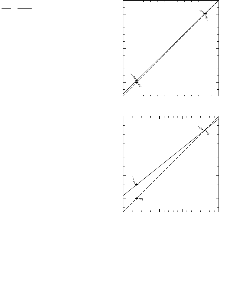
Figure 10.

Figure 10. Comparison of fractionations affecting

carbon and hydrogen. In each case, the broken line

represents a “one-to-one” approximation and the

solid line represents the accurate relationship

described by the equation. The approximation is

essentially valid for carbon but seriously in error for

hydrogen.

-15 -10 -5

, ‰

-35

-30

-25

-35.0

-34.7

P/R

= 0.980

- 20

-24.9

-25.0

, ‰

-300 -200 -100 0

, ‰

-500

-400

-300

-200

P/R

= 0.800

- 200

-200

-500

-440

D/H

Acknowledgements

Figures 1, 2, 6, and 9 were prepared by Steve

Studley. These notes derive from teaching materials pre-

pared for classes at Indiana University, Bloomington,

and at Harvard University, Cambridge, Massachusetts. I

am grateful to the students in those classes and for

support provided by those institutions and by the

National Science Foundation (

OCE-0228996).

References

Bigeleisen J. and Wolfsberg M. (1958) Theoretical

and experimental aspects of isotope effects in chemical

kinetics. Adv. Chem. Phys.

1, 15-76.

Farquhar, G. D., Ehleringer, J. R., Hubick, K. T.

(1989) Carbon isotope discrimination and photosyn-

thesis. Annu. Rev. Plant Physiol. Plant Mol. Biol.

40,

503-537.

Hayes, J. M. (2001) Fractionation of the isotopes of

carbon and hydrogen in biosynthetic processes. pp. 225-

278 in John W. Valley and David R. Cole (eds.) Stable

Isotope Geochemistry, Reviews in Mineralogy and

Geochemistry Vol. 43. Mineralogical Society of

America, Washington, D. C. pdf available at

http://www.nosams.whoi.edu/general/jmh/index.html

Mariotti A., Germon J. C., Hubert P., Kaiser P., Leto

Ile R., Tardieux A. and Tardieux P. (1981) Experimental

determination of nitrogen kinetic isotope fractionation:

some principles; illustration for the denitrification and

nitrification processes. Pl. Soil

62, 413-430.

McKinney C. R., McCrea J. M., Epstein S., Allen H.

A. and Urey H. C. (1950) Improvements in mass

spectrometers for the measurement of small differences

in isotope abundance ratios. Rev. Sci. Instrum.

21,

724-730.

Mook, W. G. (2000) Environmental Isotopes in the

Hydrological Cycle, Principles and Applications.

Available on line from http://www.iaea.org/program-

mes/ripc/ih/volumes/volumes.htm

Scott, K. M., Lu, X., Cavanaugh, C. M., and Liu, J. S.

(2004) Evaluation of the precision and accuracy of

kinetic isotope effects estimated from different forms of

the Rayleigh distillation equation. Geochim.

Cosmochim. Acta

68, 433-442.

Urey H. C. (1948) Oxygen isotopes in nature and in

the laboratory. Science

108, 489-496.